This page collects the weekly blog posts written by students over the course of fieldwork during the Fall 2022 field season. These blog posts detail each of our weekly labs, including student summaries, reflections, photographs, data, and interpretations.
Posts appear in descending chronological order, with the most recent post appearing at the top of the page.
Fall 2022 Field Season
—
Week 10
Sara Negasi and Katie Davis
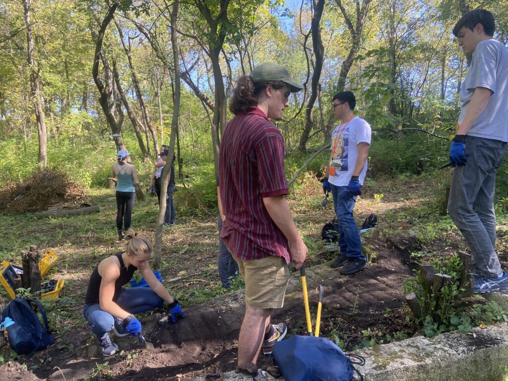
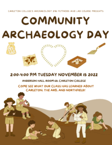
Community Archaeology Day
This week’s lab was composed of our Community Archaeology Day Event. Over the course of this class, we learned a lot about Archaeology and the methods of archaeology, as well as the history of the Olin Farm site. In our course, we also learned the importance of archaeologists learning from local community members, as they often have a much deeper knowledge of the area generally, the local history, and the community.
Our goal for this event was to involve the community as much as we could with our archaeology class. During the lab and event, we presented about our class and what we learned to Carleton students, faculty, alumni, and members of the wider community. We also had the Carleton Humanities and Arts Trailer (CHAT Trailer) parked outside our event in the hopes of further involving the community.
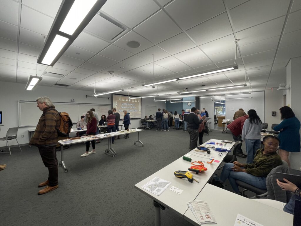
Classroom Layout


CHAT Trailer
As we said before, it’s important for archaeologists to learn from the local community, and with the CHAT Trailer parked outside our event by the chapel, we hoped to do just this. The CHAT Trailer was a place for any Community Archaeology Day guests to come and record their stories about their experiences at Carleton in the 60’s, what they know about the Olin Farm, local farming, or the Northfield community during the time of the Olin Farm, or their thoughts on archaeology and what they saw during our event. We had one guest come to share their story in the trailer, and were able to learn all about their experience in archaeology and their knowledge of the area.
Final Thoughts
Despite not having as many stories told in the CHAT Trailer, in the classroom we still heard from many alumni and community members about their memories of Olin Farm and experiences they had while at Carleton. It was valuable for us to hear feedback and personal stories from all the guests who came; we’ll take into account all that we have learned from them into our final projects and in the interpretations of our work.
We ended up having roughly 50 guests–including Carleton students, staff, and alumni, as well as community members–come by over the course of the event. With some guests being very familiar with the Olin Farm and archeology to those just then learning about archaeology and our work, it was great to see all of the students, staff, alumni, and community members coming by and showing interest and curiosity in what we’ve been doing this term. We thank all our guests for taking the time to come to Community Archaeology Day!
Recap of Week 9
Written by Ayanna Rose 🌹 + Bladimir Contreras 🌚
Nov. 15, 2022
Dear Valued Readers,

Archeology, like any field of science, follows the scientific method, so this week (Week 9), we focused on “reporting our findings” by preparing for Community Archeology day (CAD) since it is the only day we get to engage with the community and its stakeholders.
Therefore, our primary objectives for this lab were to consider how we would inform community stakeholders about what we’ve done and discovered in class and effectively communicate and present those findings with a broad range of people. More importantly, our diligent prep for CAD would consider how archeology plays a crucial role in understanding our history and helps honor it.

We began our preparation for community archeology day by selecting the artifacts to display. Groups selected artifacts based on: interest, the estimated age of each object, and the potential for further research. It was essential for us to choose objects that exemplified the group's main research area while still considering the background knowledge of potential community members coming to visit.

Moreover, objects such as ceramics with distinct patterns and artifacts with specific dates, were ideal choices for community archaeology day as they allowed groups to expand on Olin Farm history with material remains.

After groups searched for artifacts that were within specific sections of the Oiln Farm, such as the hog pen section, groups selected artifacts that were respective to their CAD project. For example, the group that specialized in Olin Farm history during 1916-1960 selected artifacts that showcased that specific time period while still keeping in mind the interest of CAD visitors. In addition, groups made sure to select objects that were somewhat identifiable or had a fascinating history. From there, groups created a curation tag, or a label, for each selected artifact to adequately describe and store them after the event. The curation tags were composed of the site name, date of excavation, and term excavated.

Interestingly enough, with the help of Google Photos and Virtual Reality (VR) software, students were able to create a more immersive experience for potential CAD vistors. This was done by a group of students who went back into the Olin Farm and took several pictutes of the Olin Farm area and used Google Photos to convert those pictures into a 360-degree experience. As a result, students could look around the site virtually and get a comparable experience to being at the site itself and were thrilled to showacse this on CAD.

Sadly, that is all the information we could report about for this week. Thank you for reading this far, we truly appreciate it. If you have any questions, comments, concerns, input, etc. regarding the entry above, feel free to reach out to us via email @ contreasb@carleton.edu or rosea@carleton.edu. We'll be more than happy to connect with you :)
—
Week 8
Dani Reynoso and Maya Shook
The purpose of our lab this week was to continue the analysis of the different artifacts we’d found at the Olin Farm site. After splitting into small groups, we were each given three bags of artifacts already classified by material (ceramic, metal, glass, etc.) and other tools to further analyze them. These tools included rulers, a scale, and different charts in order to determine their paste type and ware type.

We first started with analyzing a bag of ceramic sherds that each group had collected during excavation. Our task was to log each piece onto the artifact database spreadsheet with information such as their color, weight, sherd type, design and paste type. Something we learned in this lab was being able to identify a sherd type as either a piece of a plate or some other sort of vessel, which was very challenging once we were working on tiny pieces. We also had some practice differentiating between the different paste types such as stoneware, earthenware, and porcelain. We found this a bit challenging because a few pieces of stoneware looked and felt like porcelain, but they weren’t exactly the same texture. We were also able to piece together some pieces of ceramic but were unable to recreate an entire vessel.

Another new objective we practiced was estimating the orifice diameter of the original vessels using some of the ceramic rim sherds we found. We had this sheet of paper (pictured below) that shows different lines pertaining to different inch measurements. In order to find the diameter of a vessel, even if it wasn’t completely intact, you could line up its orifice until it aligned with one of the curves. The number above the line would be the diameter in centimeters.

We entered the information from our analysis in our artifact database, which includes data collected by the class last spring and by our class this fall. Most of the information from the ceramics collected by the archaeology class last spring had already been entered into the database; however, the diameters had not yet been measured. The data entry process for these artifacts was especially difficult because we had to match each one to an entry in the database. Since many sherds had come from the same and similar vessels, many had similar characteristics so it was difficult to match them all. This process was susceptible to human error, but we tried our best to be as thorough as possible.

After we finished with the ceramic sherds, we moved on to imputing data about other artifact classes like metal and glass. Classifying these artifacts was easier than classifying the ceramic sherds since there were less categories to sort them into and less variety of material.

After concluding our analysis, we used our data to create pivot tables. Since our database includes all the artifacts that we and the last class have found, it looks overwhelming. Using Microsoft Excel to create a pivot table displays the data so that it is visually accessible and easy-to-understand.

Week 7
Graham Gordon and Lily Akre
This week, our lab began with the class divided into two groups, with one to clean the artifacts that they had found out in the field last week and the other to begin processing the artifacts that we had already cleaned last week. The majority of the artifacts were bones, so the cleaning process was fairly straightforward. It was important to keep track of which artifacts were found where, so we made sure to keep all of the artifacts from the same bags in one area.
The cleaning process is fairly simple. Using water to clean bones can exacerbate breaking in the structure of the bone, so we used dry toothbrushes to brush the dirt off the bones. We brushed the dirt off over buckets, then placed the clean bones on trays with other artifacts from the same level. Most of the bones were fairly small, so we had to be careful not to break them. The process for cleaning glass, ceramic sherds, and all other types of artifacts was very similar, but we were able to use water while cleaning. In the picture below, you can see the variety in size and shape of the artifacts.

Fig. 1: Students cleaning bone and laying them out on paper towels

Fig. 2: Weighing a bag of metal artifacts
As for the second group, we began by dividing up our exquisite slate of artifacts among smaller groups and emptying them out, bag by bag, only so we could put them all back in(while counting the amount, of course!). Then, once we were able to acquire a second scale from the Geology department, we weighed each bag. All of this was, of course, in order to log the data relating to each bag in the archival spreadsheet.
Then, we moved on to the next part of the lab, entering data into a massive Google Sheet that looks like this:

This is where our detailed recording while excavating came in handy. All we had to do was log each bag with count, type, number, and weight. We did this so that we could systematically see and keep track of our artifacts, where they came from, who excavated them, and general information that might come in handy in the future.
After different groups finished cleaning and weighing and double-checking all of our data, we then moved on to some wonderful artifact analysis. One example of an artifact that we deemed interesting enough to analyze is this nice rusty beer can:

With some research, it was deduced that the holes on the top of the can came from a contraption called a church key, which was used for much of the 20th century to open cans with two holes, one to pour/drink from and the other for airflow.
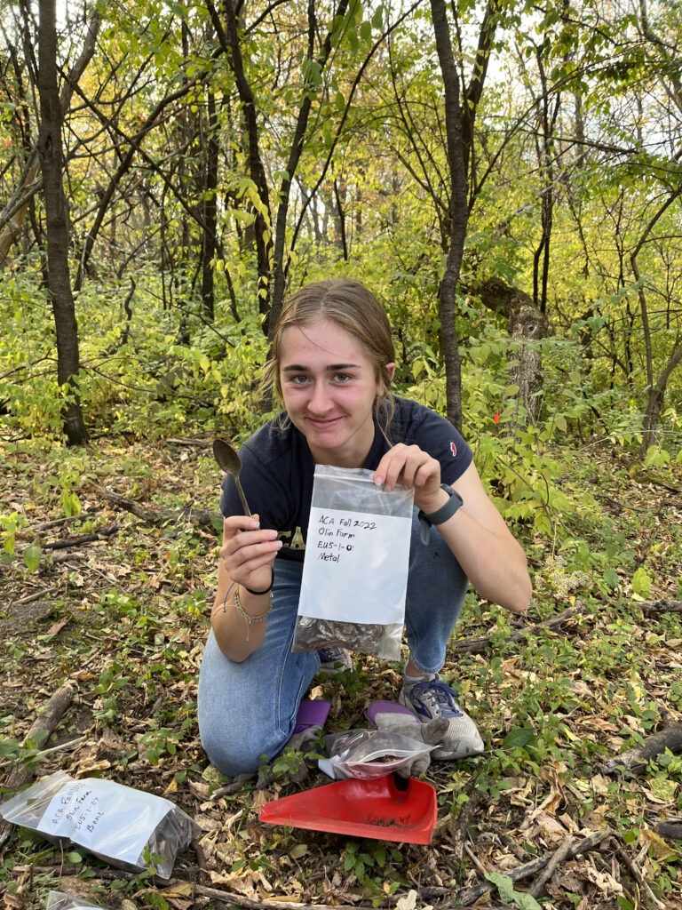
Other researchers examined some spoons, sherds, and rusted metal of various shapes and sizes. We found the concept of analogy, which we learned about during Week 6, to be quite helpful in our research. For example, I researched sherds we had found. I started off by dating the ceramic based on the maker’s mark. Then, to learn more about how the ceramic fit into the larger Carleton story we have been learning this term, I looked up other collegiate ceramics from a similar time period.
Next week, we’ll continue with our data entry of the second set of excavated artifacts, as well as zeroing in on the artifact analysis aspect while learning more about how to do so!
Week 6
Morgan Dieschbourg and Hali’a Buchal
Our lab objectives in Week 6 were to finish excavating our three units at the Olin Farm site, and begin cleaning artifacts in the lab for later analysis. A small group of students stayed in the lab, while the rest of the class returned to the excavation sites.
During the class period before the lab, Professor Kennedy provided a lecture on the interpretation of artifacts and the importance of solidifying the focus on where to dig to further understand the Olin site. Excavation groups sought to uncover additional artifacts and see whether group findings would clarify purposes of Olin Farm in terms of the presence of specific animal groups or possibly highlight more of where each building was situated.
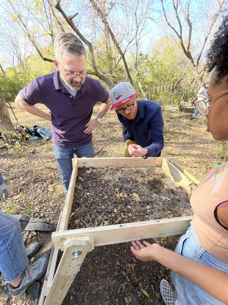
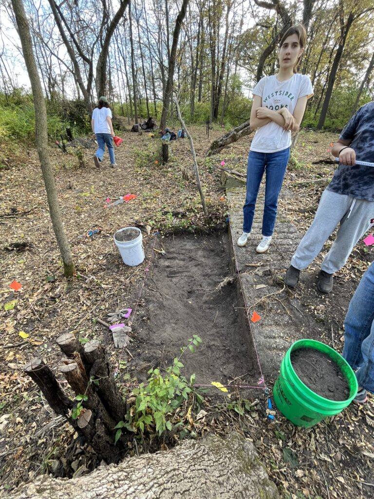
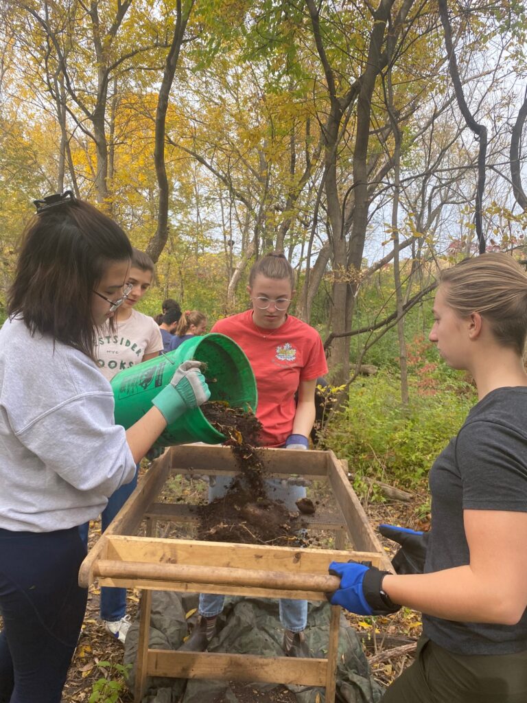
At the excavation sites, we further split into three groups, one for each excavation site. The group excavating in the hog shed area (UE8) (Image 1 & 2) continued to not find many artifacts, and so we abandoned that excavation site halfway through the lab and focused on the machine shed unit and the ceramics unit.

Image 1: The hog shed excavation pit

Image 2: Students at the hog shed unit sifting dirt removed from the pit using a ¼ inch screen
At the machine shed (UE6) we started digging level three of the pit, eventually digging down to the base of the concrete foundation. The soil became more compacted and wet the deeper we dug. We only used trowels and not large shovels, which allowed for more care and dexterity when digging around roots. Now that we had more experience excavating and the soil was more compacted, we were able to be more organized and work faster (Image 3). We continued to find lots of bones, likely from cows, pigs, chickens, and rodents. We found some larger chunks of brick and concrete near the machine shed floor, but not any large chunks of slag. We also found small fragments of charcoal in level 3.

Image 3: A student carefully digs with a trowel while others bag artifacts and take notes

Image 4: Reaching the base of the machine shed

Image 5: Students resize excavation pit to a 1×1 grid
The bone group in UE7 focused on creating a smaller, more focused site grid (avoiding the tree stump) using measuring tapes, strings that indicate the boundaries of the rectangular grid, a line level, with two perpendicular lines intersecting at the site datum point. Again the resizing of this area to a 1×1 grid aided in producing a more efficient process in excavating, collecting, screening, and labeling artifacts (Image 5).

Image 6: A student begins excavating UE7 using the side of a trowel to uncover soil level two.

Image 7: Showing process of cleaning up side walls of excavation pit
Once the excavation was dug using the side of the trowel to make sure each stratigraphic layer was exposed with caution to prevent any harm done to artifacts being uncovered, the side walls of the pit were examined for artifacts (Image 6 & 7). It is essential to clean the side walls of the excavation pit to ensure that all artifacts and features are identified and placed in buckets for screening.

Image 8: A student holding large piece of slag found in the process of excavation.
As excavation continued, the frequency of bones decreased. We found ceramic sherds, glass shards, nails, and other metal (potential machine parts). Once the bone group transitioned into level 3 of the soil layer, there was an overwhelming amount of slag (stony waste leftover from metal smelting and welding) (Image 8), found under the bone, which raises the question: what caused this large amount of slag? Could its presence be a result of metal work given the proximity to the machine shed?

Image 9: Students in the bone group (responsible for UE7) screening artifacts found during excavation.

Image 10: After screening, artifacts are identified and sorted by type into sample bags to bring back to the lab.
Through the process of screening (Image 9 & 10), we found that ceramic sherds, glass shards, and bone all were mixed and found in each layer. So with this idea, we inferred that the mixture of these artifacts was possibly the result of a relocation of animal remains and other artifacts into a mass dump into the area where we excavated. We would like to further analyze the mixture of bones to determine what animals they belonged to, and which bones have evidence of tool marks. This analysis would add to our interpretation of the previous owners of Olin Farm, what animals they may have kept or had access to, and their methods of distributing animals bones and other garbage.

Image 11: Form used to record details of each strata layer and artifacts found in each layer (this one for UE7).
Recording aspects of the excavation unit, such as change in soil texture, number and type of artifacts found, etc. (Image 11) is beneficial for later data interpretation.

Figure 1: GIS map of the Olin Farm site, showing points mapped by the Trimble outlining important features.
The Trimble group (UE8) made efforts to identify the outline of the barn by marking artifacts found using the Trimble GNSS/GPS system that were thought to be associated with the barn. As depicted in the GIS figure above, this group made efforts to identify and mark artifacts to indicate the potential location of the hog shed but did not have much success. Also in Figure 1, the outline of the machine shed and its wall is clearly mapped using the trimble which can help in producing clarity surrounding the building locations.
Back in the lab, students used toothbrushes to carefully clean the dirt off of artifacts. Artifacts like ceramics, glass, and plastic were easier to clean because they could be scrubbed with water, but bones had to just be dry brushed, as water could damage the bone.
The last task involved covering each excavation unit with a tarp to preserve the progress we made and protect the pits from weather. If we need to return to the Olin Farm site to answer a specific question or cross reference where an artifact was found, the site would still be somewhat protected. Next week the group that was excavating will be working in the lab cleaning artifacts, while the former lab group will begin entering the data collected into the computer.
Week 5
Somin Sarno and Yikang Bin
After weeks of learning how to map, survey, and shovel test a site, we finally did what people typically consider when they think about archaeology–excavation! Our focus in this lab was continuing our exploration of the machine shed, a place in Olin Farm probably used in its time as some kind of hotspot for housing farming equipment for the Olin family and a place to put butchered animal bones, perhaps from the nearby hog and cow farms. Given the vintage artifacts, including 50’s toothpaste tubes and 70’s dining ware, and after talking to some alumni, we think that this place also served as some kind of hub for students to hang out in after the machine shed was no longer used for its original purpose. Excavating small portions of the machine shed site gave us a lot of evidence supporting our hypotheses about the various uses of the machine shed throughout its history.
As archaeologists who want to neatly keep track of our finds, the way we divided our labor had to be organized and systematic. In our lectures and readings, we learned that there are many ways archaeologists ensure that they are carefully maneuvering and keeping track of a site and what they find there. There is the method of using computer software like ArcGIS to visualize and section our location through digital mapping, using flags to mark squares of land we’d like to explore, screening dirt we dig in case there are artifacts in the soil, and putting what we find in plastic bags with labels. The new method we discussed for this lab included the Harris matrix (figure 1), a visual diagram for the kinds of soil surrounding objects we find as we dig.

Before excavating, our class practiced making our own matrices given pictures of soil layers. We found that, depending on the student, there are many ways of interpreting and organizing layers of soil, but that the main purpose of doing so was to make sure we were keeping track of our finds in an organized way. Making matrices would help us later when we want to check what kind of context or environment an artifact was from.
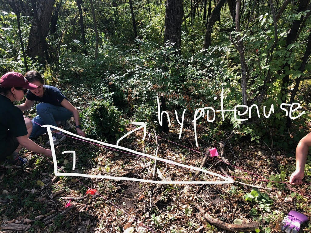
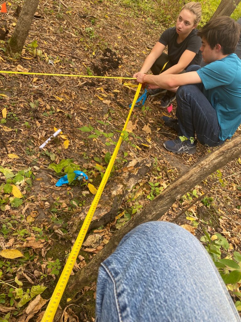
When it came time to excavate, we used tape measurers to measure the height, length, and hypotenuses (Figure 2) of the excavation units and used line levels to see how flat the units were from the ground surface. To mark our measurements, we cut and tied colorful strings to identify the boundaries of our excavation units (Figures 3 and 4). The way we chose our excavation units was based on what we thought would have the most artifacts based on our observations from previous labs, as surveying showed that there were more artifacts on the surfaces of the places we chose to excavate, suggesting we could find more underneath. Then we used a variety of excavation tools – shovels, trowels, brushes, and buckets – to start digging up the first strata (i.e., soil/rock layers) to see if our finds aligned with our initial assumptions of what we thought would be in our units.

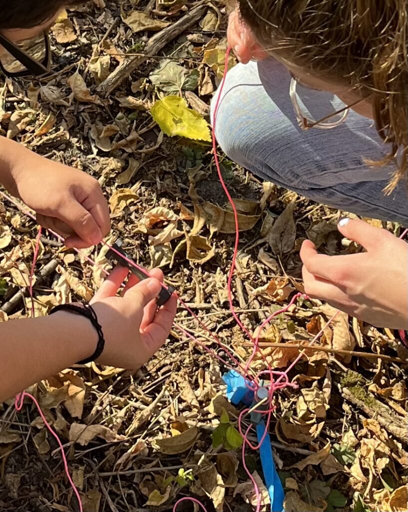
Our method of digging was to dig the soil using the sides of our trowels and to use the trowels’ sides instead of jabbing the dirt with them helped us be more cautious about peeling each stratigraphic layer–like how one would peel layers of a carrot–to keep track of the layers. In between layers, we took pictures of the newly dug levels, screened the dirt for each dig, and collected artifacts in separate plastic bags. We kept track of the layers and the objects we found in them using sheets where we described the soil, the tools used and a “plan view,” which unlike a vertical drawing which would tell us what we find as we dig down into different strata, this kind of drawing shows what artifacts we find on a horizontal plane, or their arrangement on a layer (figure 5). The tool we used for screening was a screen with 1/4 in mesh holes, which you’ll notice from previous lab summaries is a common tool we use in archaeology (figure 6).

In one of our units, we thought there would be more ceramics in it from seeing ceramic sherds on its surface in our surveying lab, but digging this area produced far more animal bones than we’d initially assumed. Given their size, these bones were likely from hogs or cows. Accompanying these bones were spoons and other dining ware, like an old glass cup with a Carleton logo on it (figure 7). We think it’s interesting to see animal bones and dining ware in the same stratigraphic layers, as their placement could suggest that the people of the 50’s or 70’s, depending on the exact dating of the dining ware, intersected with the consumption of hogs and chickens in the area. The impact that these animals had on people using the machine shed is not clear to us yet, and we don’t want to make any totally unrelated assumptions. But we still think that this find is interesting in contextualizing the machine shed and understanding how important it is to keep track of our finds in a structured way, giving us clues about how artifacts are grouped in an archaeological chronology.
Compared to other units, the one with dining ware and animal bones had the most artifacts. In other units, we found concrete pieces that were probably part of the machine shed and large chunks of slag, which is a solidified form of stone waste produced by smelting or furnaces, a sign that metal work might have taken place at this site. These artifacts came in larger numbers the deeper we dug. Although pieces of rock were not as interesting to us as the bones and dining ware since they were not as unique in their appearance and connection to people in the past, what we learned from this lab and as curious archaeologists is that any artifact found in excavation is still important. Perhaps the large abundance of slag towards the bottom of our units suggests different deposition events. More concrete pieces might suggest the machine shed floor is at the bottom of where we’re digging. We have yet to figure out the meaning behind the number of rocks at the bottom of our units, and we look forward to finding out, hopefully, in the coming labs. In the meantime, we covered our excavation units with tarps for protection from animals and people who might come to our site, as well as snow and rain, and we will revisit these units next time (Figures 8 & 9).

Week 4
Bianca Lott and Zoe Heart
Week Four’s Lab focused on learning to use and perform data input on ArcGIS (a mapping and analysis system used to make maps, analyze data, and share and collaborate), conducting shovel testing, and picking out excavation sites.
We began class first by meeting in the classroom and lab for an hour-long training session on how to use ArcGIS. This is a system that allows users to create maps with specific overlays and data inputs as well as easily analyze and visually look at data.
After last week’s surveys of both the baseball field and the Olin Farm site, we had a lot of information on survey forms that were ready to be digitized. Prior to class, Professor Kennedy and our TAs had set up a map with overlays of the specific boundaries we had surveyed. Students split into the same three groups as in week 3 and then used these maps to enter the data they had collected last class (see Figure 1). All artifacts were arranged by artifact classification (botanical, brick, ceramic, glass, lithic, metal, plastic, slag, tile, and other) and then entered into the corresponding survey area they were found in (see Figure 2). We also spent some time generating different visual interpretations of the data on the maps (see Figure 3).

Figure 1

Figure 2

Figure 3
Next, we collected our gear from the lab and moved outside to the Olin Farm site. Here the three groups returned to their respective rows to begin shovel testing. Each group dug one test pit in the center of each one of their survey squares (see Image 1). These test pits measured roughly 50cm in diameter (see Image 2). All the contents from the surface of these holes as well as all the displaced dirt were collected into buckets to be screened.


Once each test pit was dug to satisfaction, all of its contents were brought over to the screening station. Here students poured the buckets onto screens and shook the screens so that all excess dirt was removed (see Image 3). The remaining contents were then thoroughly examined to ensure that all artifacts were found.
These artifacts were then sorted by class and counted. Unique artifacts and sample groups for common artifacts were then collected in plastic bags and labeled to be brought back to the lab (see Image 4).
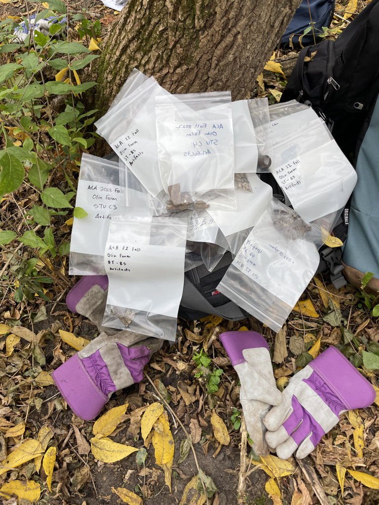
Image 4
The last task we completed was choosing and measuring a future excavation site. We chose a 2-meter-long site next to the remains of the entrance ramp to the Machine Shed (see Image 5). We decided on this site for excavation because of the likely high foot traffic of the area during its time in use which should hopefully correlate to a concentration of artifacts. To ensure that the excavation site was properly measured, we measured each side from multiple angles and cross-checked using the Pythagorean theorem (see Image 6). The boundaries of this excavation site, as well as the location of each test pit, was recorded with the Trimble GNSS/GPS (see Image 7). This data as well as all of the artifact logging will be organized and digitized back at the lab at a later date.
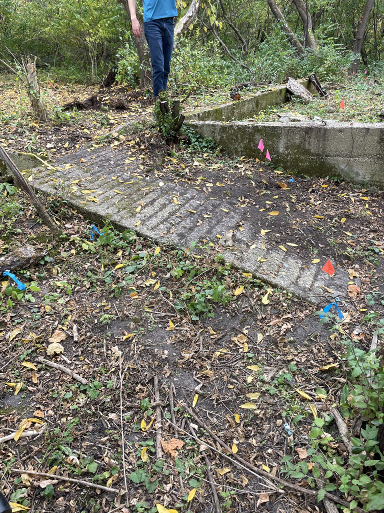
Image 5

Week 3
Chris Melo and William Johnston
In our Week 3 lab, we focused on both learning survey techniques and applying these techniques to the Olin Farm machine shed site. By the end of the day, we had been introduced to the randomized, high-probability, and systematic methods of ground survey, had learned how to fill out a survey sheet properly, and had completed a full systematic grid survey of the machine shed.
During our class period, Professor Kennedy gave a lecture outlining the three main types of archeological survey: randomized, in which survey locations are picked, as the name suggests, randomly, high-probability, in which the archaeologist surveys those places they believe are most likely to contain useful information, and systematic, in which the site is surveyed through a standardized pattern such as a grid or a series of lines.
The lab proper began with a brief introduction to survey forms before we walked over to the baseball field. There we used a tape measure to divide the field into four equal squares in preparation for a transect ground survey.
The goal here was to practice survey techniques (careful study, properly completed survey forms) in preparation for our “real” survey of the machine shed later in the lab. Having divided the field into squares, we all lined up against the far wall and began to slowly walk forward, scanning the ground for artifacts. We marked every artifact we found with a flag, returning later to note them down in our survey forms. By the end of the survey, we had not only cataloged nearly every artifact on the baseball field, but had obtained a working understanding of survey techniques. (In terms of the actual artifacts discovered, most were either plastic zip ties or sunflower seeds, though we did happen upon a small animal bone.)

Having completed our practice survey of the baseball field, we moved on to the machine shed site. Here we employed a more complex survey methodology than what we had used on the baseball field. Before our arrival, Professor Kennedy had divided the site into three rows of five-meter squares, with the first row, A, having four squares and the next rows B and C each having six.

On arrival, we split up into three roughly equal groups, designating one member of each group as the “crew-chief.” The groups then went down each row, methodically inspecting every square before moving on to the next. The “crew-chief,” meanwhile, took notes and pictures of each artifact we discovered. The reasons for this change in methodology from the techniques we employed in the baseball survey are two-fold. First, the machine shed site possesses a much higher volume of artifacts than the baseball field. Had we simply walked forwards in a line, we would have missed some artifacts and could have become disorganized as some students stopped for many minutes to catalog their finds. Second, the forested terrain of the machine shed makes it very difficult to walk forward in straight lines or to establish clear lines of sight as we had on the baseball field.
By the end of our survey, we had discovered a wealth of artifacts around the machine shed site. These artifacts were mostly concentrated around the machine shed foundation in squares B1 and C1 and in the trash pile in squares B4 and C4. Metal slag, paving stones, and bricks were the most common artifacts we encountered along with smaller quantities of glass, metal construction material, and pottery. Some of our more interesting finds (figures 4 and 5) include a fragment of a moisturizer bottle and a shard of pottery from what was likely a uniquely large vessel.
In sum, this lab succeeded in not only furnishing us with a basic understanding of surveying but also allowed us to obtain a clearer picture of the artifact distribution at the Olin farm site, information which will be of tremendous use when we begin the next portion of our investigation: the excavation.


Week 2
Kaija Maier
The primary focus of Week 2’s lab was to learn how to map and investigate an archaeological site prior to collecting artifact data (sometimes called “site reconnaissance”). We learned how to use GNSS (global navigation satellite systems) and how to identify surface artifacts such as glass, metal, ceramics, and butchered animal bones. We also focused on clearing vegetation, brush, and forest debris from building foundations and future excavation locations.
We began the lab by first meeting in the classroom and learning about GNSS. It was here that Wei-Hsin Fu, the Director of Carleton’s GIS Lab, went over basic mapping with us, in addition to how to use and understand GNSS and GPS (Global Positioning System) to map archaeological sites. We will use a handheld GNSS from Trimble, called GeoExplorer, to collect data this term. After learning how to use the handheld devices inside, we practiced taking points and lines on Carleton’s campus. After a brief period of practicing, we brought ourselves and our tools to the Olin Farm Site where we began surveying the surface and uncovering more of the machine shed. The members of our class spread out across the chosen site and began to clear away the thin layer of dirt and weeds covering the walls and floor of what was once the machine shed. The goal of this lab was to begin finding the boundary of the building, in order to gain a better understanding of how this space was used.
Our class spent much of the time uncovering a cement ramp that was part of the machine shed (Figure 1). In doing so, we discovered many artifacts and features of interest. This included metal door hinges and even some baby mice! When something was found, it was marked by students using a neon pin flag, so as to make it easily identifiable when we come back to the site next week. We also took time to walk around the site and found and marked the location of many partially hidden pieces of broken ceramic and glass (Figures 2 and 3). We were able to uncover many feet of concrete flooring in the machine shed, which went much further back into the trees than we thought was possible. We marked the edge of this flooring with a line of flags and hope to finish uncovering it during our next lab. We will also look at historic insurance documents from 1941 that list the size and dimensions of the machine shed, to estimate the portion of the shed that is still uncovered (see Figure 4). We left the site at the end of the day covered in pin flags, awaiting further study.